Highest ever rise in carbon dioxide levels

https://www.newscientist.com/article/2079995-highest-ever-annual-rise-in-carbon-dioxide-levels-recorded/

This rise that we see here is an annual rise in the concentration of carbon dioxide in the atmosphere. This extra rise over and above the normal seasonal cycle is what was expected and which I discussed previously here  and my previous post on Indonesian fires whereby I clarify that we have a trend in rising CO2 due to human-induced emissions, we have a seasonal cycles due to changes in photosynthesis and decay and we have these extra wiggles due to changes in rainfall and photosynthesis due to the El Nino (or changes in the ENSO cycle). These extra increases in CO2 would generally follow or lag the changes in sea surface temperature associated with the El Nino as explained in the link here.

I first became aware of these changes that would allow one to predict such changes as we see described in the New Scientist post above a few years ago ironically not from main stream scientists but from contrarians. This was my first real experience of climate contrarians. . I realized the reasoning from these contrarians was flawed and later found the explanations regarding the ENSO cycles from main stream science as indicated in the previous link.

So what where these contrarians (Spencer and Humlum) attempting to explain. Rather than explain the obvious and accepted facts that Humans are the main cause of increasing CO2 in the atmosphere and this trend in rising CO2 was causing rising trends in both sea level and temperatures, they played with the data to try and see if they could show that it was rising temperatures that was causing the trend in CO2 to rise. There is of course nothing wrong at looking at different ways to analyse data but what was clear is that the obvious was overlooked and the inferences or conclusions were flawed. Their manipulation of the data effectively removed the trend and the seasonal cycles and so their conclusions could have nothing to do with the trend. Without apparently realizing it they were looking at the variations in CO2 lagging the changes in sea surface temperatures, SST,  associated with the ENSO cycle and then trying to make connections between the rise in the trend of CO2 and the rise in the trend of temperatures.

The connection here regarding these variations is changes in SST and wind patterns to changes in ocean circulation and large scale wind patterns to changes affecting precipitation and photosynthesis and to these producing the extra changes in CO2 that we note today towards the end of the ENSO pattern.

Shaviv made the same mistakes in trying to associate changes in SST and sea level rise confusing cause and effect.

Indonesian Fires

Typically During El Nino years we see forest fires that will raise the CO2 concentration levels in the atmosphere.

https://www.washingtonpost.com/news/energy-environment/wp/2015/10/15/how-indonesias-staggering-fires-are-making-global-warming-worse/

These Indonesian fires will contribute towards this effect although the causes of the fires are not completely natural as explained in the post above.

Contrarians in the past and undoubtedly in the future will use the data (CO2 concentrations increased due to these CO2 pulses) to arrive at false conclusions.

These fires cause atmospheric CO2 concentrations to rise more than would be expected from emissions alone. It is this extra rise in CO2 that LAGs variations in SST that have led Humlum, here and led Spencer, here, in the past to wrongly assume that SST are the cause of CO2 rise in the overall trend of CO2 rise. The overall trend in CO2 rise is of course caused by human emissions.

It was to be expected that something similar would happen during an El Nino as discussed, here, It is also likely that we will see more events globally in the short term(over the next few months) that will further contribute to short term variations in this upward direction.

Inevitably these anomalous upward variations in SST will decline, La Nina will return, global rainfall over land will increase, plant growth will increase and the trend in CO2 concentrations will rise less steeply. (This offset due to this reduction of CO2, however, will not fully compensate for the rise in CO2 during El Nino in the case of these Indonesian fires as explained in the news article at the top of this page). Again the variations in CO2 will lag the SST to be misinterpreted by climate contrarians. 

Roy Spencer’s “model”

Carbon dioxide and Sea surface temperature.

Roy Spencer plays with data in a failed attempt here.  He attempts to explain that the rise in atmospheric CO2 has mainly come from rising sea surface temperature, SST.

 I only recently came across Spencer's blog though it was written back in 2009 and thought it relevant to discuss this in light of the present El Nino of 2015. The relevance is discussed here.

A coherent and consistent explanation is generally accepted for the rise of CO2 since the start of the industrial revolution. This explanation includes the causes for the trend in CO2 and different causes for the variations in CO2. There is little doubt that the trend is caused by human activity and in particular the burning of fossil fuels.

There is continual movement back and forth between the atmosphere, biosphere and oceans; however these are net fluxes that are indicated.

In spite of the oceans warming, the oceans are net absorbers because of the extra CO2 pressure from the atmosphere

Roy Spencer challenges this and while not stating his conclusions explicitly he makes strong implications:-

http://www.drroyspencer.com/2009/05/global-warming-causing-carbon-dioxide-increases-a-simple-model/

According to Spencer something is causing SST to increase and this is most likely to be due to changes in cloud cover for reasons unknown and the cloud cover conveniently changes at a level too small to measure. Spencer suggests this change in SST is the main cause of CO2 to rise in our atmosphere. To arrive at this viewpoint Spencer uses a circular argument assuming it is true in the attempt to show it is true. This logical fallacy on its own shows his argument to be false but Spencer also requires mutually exclusive arguments in an attempt to justify his arguments. Playing with data, Spencer makes a “model”, (it is hoped he is not equating this to resemble anything like a climate model) which is nothing more than an algebraic equation to which he quickly finds a solution.

Confusing the causes of trends with the causes in natural variation and confusing correlation with cause, Spencer then makes a provocative claim that if scientists don’t take this incredulous flawed argument seriously then they must be politically motivated for doing so.

Perhaps Spencer’s main flaw (although all the flaws are in fact fatal to a coherent argument) is that any dubious conclusion he makes as to causes in natural variations he assumes are applicable to the causes for the trends. While attempting to consider some of the intricacies of natural variation he makes simple fatal errors on explaining the simple basics. The complexities of the variations are interesting and well worth investigating. (A repeat of the link above is given here which contrasts much with Spencer and explains the significance of the lag that Spencer refers to). Rather than trying to clarify these complexities Spencer uses them to obfuscate the simpler basics.

Spencer’s mutually exclusive arguments.

Roy Spencer disagrees with the diagram above. He doesn’t dispute the fact that the atmosphere has been increasing in CO2 and presumably he doesn’t disagree that we have been burning fossil fuels. So the top line in figure 1 is not disputed, give or take a little uncertainty.  What Spencer disagrees with is the net fluxes represented by arrows b and c into the biosphere and oceans and furthermore he disagrees with their direction.

He cannot make up his mind if arrow b or c should be reversed. For obvious reasons both cant be reversed or the atmosphere would gain more than humans emitted.

He would like to argue the “Coke-Fizz” effect ( arrow c reversed), the argument that warming oceans would give up their CO2 due to them being warmer, but he knows this argument is flawed so he jumps to the other argument that the biosphere could be net sources of CO2 to the atmosphere but knowing this is also flawed he leaves it vague which of these mutually exclusive arguments he proposes.

If the oceans were net sources of CO2 (arrow c reversed) then we would require more greening (arrow b to be most of the 10 Gt /year) and the oceans to be increasing in pH (or becoming more alkaline, which is not observed)

 The evidence of carbon 13 isotopes falling excludes the possibility that the oceans are the sources of CO2 to the atmosphere. Plants preferentially take up C12 and the oceans being the source would prevent the C13/C12 ratio in the atmosphere falling to the extent for which there is observational evidence. Aware of this Spencer “pre-empts” this argument by switching to the biosphere as a net source. He states that “the C13 change is not a unique signature of fossil fuel source”. This is true but is an example of a half truth. Spencer fails to acknowledge that the reduction in C13/C12 ratio completely destroys his previous argument that the oceans via the “Coke-Fizz effect“could be the source of the atmospheric CO2.

The biosphere being a source for the CO2 could explain the C13/C12 ratio; however he doesn’t dwell on this for long. This would mean the biosphere was ungreening ( he has argued on other posts that a benefit of burning fossil fuels is that it is causing greening of the atmosphere) and the oceans would be gaining most of the 10Gt/year of CO2. 

It would appear that you are to momentarily believe that the oceans could be the source for CO2 and if you find a flaw in that argument you can perhaps believe the biosphere is the source. Not only are both these arguments flawed but they are mutually exclusive unless you think that mass can somehow not be conserved.

Spencers Circular arguments.  Spencers Model.

Spencers “Model”

delta[CO2]/delta[t] = a*SST + b*Anthro

This claims that the CO2 gradient correlates linearly on a combination of SST anomalies and an anthropogenic component.

Is Spencer implying that his “model” based on a simple algebraic equation is supposed to be a replacement for sophisticated climate models that use scientific laws and data coded into computer language to obtain emergent weather patterns? One gets the feeling he is hoping climate contrarians will infer this.

It is inconceivable that CO2 concentrations are proportional to an anomaly based on differences compared to a 1961 to 1990 average.

The value for SST anomaly depends on what years we compare SST to. SST’s are compared to the average of years 1960 to 1990. So the solutions for the co-ordinate values that fit a narrowly defined period with a start and end date depend on this choice. This means that Spencer decides how much is SST (which he calls natural) and how much is anthropogenic based on this arbitrary choice.

http://www.drroyspencer.com/wp-content/uploads/simple-co2-model-fig06.jpg

If the model is extended into the future, as long as CO2 emissions occur and absolute values of SST increase, then the gradient of CO2 concentrations will increase. This will mean an inevitable exponential increase in CO2 concentrations that would indeed imply drastic positive carbon feedbacks to carbon emissions. Any SST would mean that CO2 concentrations would rise without any emissions. Thankfully the model is flawed; the exponential effect is seen in the graph above.

The observed CO2 and the model are made to fit in year 1958 and then this formula is used to calculate how the model changes over the time period. The coefficients a and b are “solved” to give the best fit. The solution favoured by Spencer results in the atmosphere at the present time gaining about 1Gt/year (10%) from anthropogenic sources and hence 3.5GT from “natural sources” due to SST rise. He doesn’t really explain where the other 9GT of human emissions goes.

In his original graphs the anthropogenic component didn’t seem to fit well because he decided to plot the rate of change of CO2 against time and depending on how little the data is smoothed you can get wild fluctuations with this technique. This is a common technique used by an obfuscator when they want to show something that is well correlated not to be so.  He didn’t use that technique when he wanted his 90% “natural” plus 10% anthropogenic to fit well.

For an explanation of the variations of CO2 associated with ENSO cycles along with references see here.

Variations On the rate of change of sea level rise

Global warming due to the build up of greenhouse gases, primarily carbon dioxide (CO2), causes the sea level to rise.

Here I will describe a flawed attempt by Nir Shaviv at attributing global warming on changes in solar activity. This case by looking at sea level rises rather than surface temperatures.

Shaviv posted to the Financial Post on June 16 2015 claiming “the sun raises the seas”. In that post (link to follow) he claims he has evidence to show that it is changes in solar activity that is the major factor in present day sea level rise. However his arguments do not disprove the consensus view that this sea level rise is primarily due to the enhanced Greenhouse Effect (GHE) due to human activities. It is however reasonable to consider sea level rises as most of the energy built up due to Global Warming is taken up by the oceans. It is this energy absorption that results in sea level rises.(figure 1)

Figure 1 Sea level rises CSIRO

https://commons.wikimedia.org/wiki/File:Trends_in_global_average_absolute_sea_level,_1880-2013.png#/media/File:Trends_in_global_average_absolute_sea_level,_1880-2013.png

If this sea level rise could be attributed to changes in the sun rather than greenhouse gases then this would be a way of undermining the GHE.

Previous attempts at showing that it is changes in the solar activity that has caused surface temperatures to change have failed:-

http://skepticalscience.com/solar-activity-sunspots-global-warming.htm

http://skepticalscience.com/solar-cycles-global-warming.htm

To raise the sea levels requires extra energy; energy obtained via the GHE. Most of this energy raises the temperature of the sea and cause the seas to expand. Some of the energy also results in net melting of land ice that also raises sea levels. This explains the trend in rising sea levels. The short term variations, however, may be due to natural variations such as changes in solar activity or in oceanic circulation patterns such as El Nino and La Nina; the later resulting in changes of rainfall and snowfall over land changing the amount of water removed from the oceans.

However Shaviv claims that the sea level data shows.....the rate of change of sea level “follows the sun”.....and then concludes that it the sun that it is the cause of sea level rise.

I will argue that the first point is very dubious but also show that even if it where the case the calculations he shows about rates of changes of sea level does not support the conclusion. Shaviv doesn’t explicitly say he has made the conclusion from that evidence, however in his post that is the only evidence he presents and so the very strong inference is made.

Figure 2 Shaviv

http://business.financialpost.com/fp-comment/carbon-week-the-sun-raises-the-seas

The lower graph in figure 2 shows sea level rises without uncertainties but otherwise similar to that of figure 1.

The upper graph shows the rate of change of sea level (blue line) and variations in solar flux (black line). We see these two superimposed graphs overlap well with similar amplitude phase and frequency and so superficially it may seem that the conclusion follows.

Let us assume for the moment that the rate of change of sea level follows the sun as in the upper diagram of fig 2 is true. Why does the conclusion not follow?

When manipulating data to tease out underlying causes, it is important that your conclusions are not really a result of the manipulations and not the data itself.

Shaviv manipulates the data by effectively removing the trend in sea level (explained later) and smoothing out the sea level to omit seasonal changes so he is only left with other natural variations. Nothing wrong so far. However one can no longer make conclusions about the solar activity and the trend in sea level rise but this is precisely what he seems to do.

Shaviv does not actually remove the trend; he simply hides it. If he were to remove the trend and the seasonal cycles we would be left with variations that would be more obviously related to ENSO cycles. Instead he finds the rate of change of sea level suitably smoothed so that a linear trend will be seen as a horizontal offset so when compared and plotted with another graph showing the solar cycle with an independent scale and origin he has effectively removed the trend for comparison purposes.

Perhaps simpler examples can clarify this and this is good reason to look at what is regarded as the main cause of modern day sea level rise.

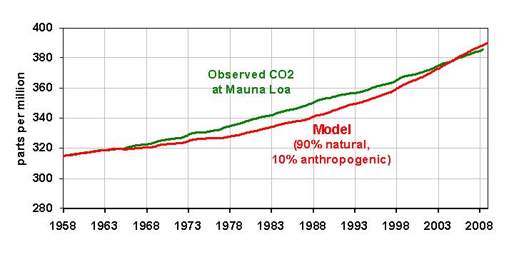
Keeling curve:-

Figure 3 CO2 levels

https://commons.wikimedia.org/wiki/File:Mauna_Loa_CO2_monthly_mean_concentration.svg#/media/File:Mauna_Loa_CO2_monthly_mean_concentration.svg

This diagram plots the CO2 smoothed out to show the monthly changes (red curve) and yearly changes (blue curve). The monthly changes are due to the seasonal cycle whereby CO2 is absorbed by plants during the growing season in the NH and CO2 is released by decay over the winter months. The trend is due to the build up of from human activities mainly in the burning of fossil fuels.

When focussing on the rates of change, the annual rate of change of CO2 is completely dominated by the monthly rate of change clearly because the slow annual trend is smaller than the swings in concentration over each single year. A graph of the rate of change of the monthly concentration of CO2 would show positive and negative swings across the time axis off-set slightly due to the long term trend. (Similar to figure 4).

This Keeling curve can be approximately modelled by a straight line with a long term trend rate (given the value k) modulated by a sinusoidal wave.

CO2 = kt + asinwt + a constant

Rate of change of CO2 (wrt to t) =  k+awcoswt

Figure 4 rate of change of idealized CO2 concentration against time.

Figure 4 shows a sinusoidal wave with an average value k, that is offset by a value k, the long term trend rate. The higher the frequency, w, of noise or short term variations then the more the long term trend k is obscured by the amplitude, aw.

From the Keeling curve we can see that the rate of change of the CO2 concentration (as seen by the changing slope of the red graph) mainly follows the seasons but this is totally independent of the causes of CO2 build up due to human activities as seen by the long term trend.

Back to sea level rise:-

 Shaviv has smoothed and sampled the sea level data at appropriate intervals, just enough but not too much, ensuring the short term variations dominate the trend when looking at rates of change. (....too little and other variations would dominate the solar cycle....too much and variations over frequencies comparable to the solar cycle would disappear).

However what about the similar frequency and amplitude of the rate of change of sea level rise and solar flux as in the upper diagram of figure 2?

The frequencies are similar partly because they are chosen to be so by deciding how much smoothing is employed and partly because there may be some albeit small connection. However I can see about two or three times per decade (when looking at the sea level rise as in the lower graph of figure 2)  when the rate of change of sea level rise should swing between positive and negative which is not reflected in the upper graph.

The amplitudes are equally similar because again they are chosen to be so....the two graphs have independent scales and further the origin of each graph is changed so that the long term trend (k, of about 2 or 3 mm/year as seen in the average of the rate of change of sea level..blue graph) is overlapped by the solar flux.

The important conclusion I make here is that any resemblance of the rate of change of sea level rise to the solar variations have no bearing on the long term trend of sea level rise just as in the case of the CO2 variations. The causes of the short term variations and the long term trend in each of these graphs are different.

There is an obvious correlation here of course, and that is the consensus view, that the long term trend in CO2 is not only the cause of the long term trend in sea level but the correlation between them is excellent (graphs 1 and 3). Shaviv has discarded the obvious and made claims or inferences that could lead the reader to a false conclusion. 

Atmospheric CO2.

By Pat Hackett

How much has CO2 risen in our atmosphere due to anthropogenic (the result of human activity) causes? This question is quite straightforward to arrive at a reasonable estimate but it is interesting to see the attempts to arrive at quite meaningless and far off estimates. This flawed method here is one by T.V. Segalstad who ignores the effects of fluxes of carbon between the oceans, biosphere and atmosphere when looking at carbon isotopes in the atmosphere.

However first some basic facts:- 

Changes in CO2 from preindustrial times to 2014.

Pre industrial CO2 levels had been relatively stable for several hundred years at around 280ppm and have risen since then to around 400ppm. Accurate measurements for over 50 years form sites such as Mauna Loa show the increases since 1956. (figure 1)

Figure 1:- Increase in CO2.

Figure 1 shows the net annual variation in CO2 due to exchange of CO2 between the atmosphere and mainly the biosphere which, over a single year, is much greater than the annual but steady increase in CO2 due to anthropogenic emissions. This annual cyclic variation can be attributed mainly to the growth and decay of organic matter in the Northern Hemisphere.

Unless volcanic activity has increased by something in the order of 50 fold, waiting for the industrial revolution to start doing so, it is reasonable to assume that the steady increase has been due to anthropogenic causes. 120ppm out of 400ppm represents 30% due to anthropogenic causes

.

How can a reasonable estimate of around 30% be changed to a range of estimates from somewhere between 0 and 4%? You may stumble across statements like this in some web sites.

Here is a link that deals with the following issue:- The Amount of Non-Fossil-Fuel CO2 in the Atmosphere-

http://www.co2web.info/hawaii.pdf

 and thus T V Segalstad arrives at the following conclusion:-

"At least 96% of the current atmospheric CO2 comes from non-fossil-fuel sources."

Does this address the same question as:-

How much has CO2 risen in our atmosphere due to anthropogenic causes?

T V Segalstad would like you to think so and numerous other web sites/blogs by the same author and others use the confusion to make further flawed conclusions. For example:-

“Hence for the atmospheric CO2 budget marine degassing and juvenile degassing from e.g. volcanic sources must be much more important, and burning of fossil-fuel and biogenic materials much less important, than hitherto assumed”.

This later cautiously worded conclusion follows on from a misinterpretation of the first conclusion.  The first conclusion (At least 96% of the current atmospheric CO2 comes from non-fossil-fuel sources.) in the above article may or may not be accurate. That is not the issue that I take up here, however it may appear to lead to the (false) conclusion that our atmosphere has only risen by 4% due to anthropogenic causes.

The flawed argument.

First an analogy.

A bank note analogy:-

Imagine you deposited £100 notes in your bank and went back a week later to withdraw your money and the cashier apologized and said only £4 of your original notes were left in your branch of the bank so you can only withdraw £4.

Surely this is not the mistake the author makes with the distractions of using the science of carbon isotopes ratios? Yes the analogy is incredibly quite similar and yet with this mistake, and a few others on the way, other false conclusions regarding the half life of CO2 in the atmosphere and the % contribution of CO2 to the greenhouse effect are then obtained. The confusion and false conclusions are carried forward to another article by the same author, and can be read in the following link.

http://www.co2web.info/

Pre industrial global carbon reservoirs.

These are given in figure 2 below. The main point here is that the reservoirs in the biosphere and the oceans are much greater than the atmospheric reservoir.

Figure 2:- Global carbon reservoirs.

The short term carbon cycle.

The short term carbon cycle deals with the movement of carbon between the atmosphere, the ocean and the biosphere. (The long term carbon cycle concerns the movement of carbon from volcanic activity as a source and the sinking of carbon by both weathering of rocks and the smaller but significant burial of organic carbon).

Figure 3:-  Pre industrial carbon.

Exchange of carbon between the atmosphere and the biosphere and oceans is continual and daily which is many times greater than the additional rate of CO2 from fossil fuels over a single year.  This exchange is partly indicated by the net annual cyclic variations that you can observe in figure1 above. However in relatively equilibrium conditions (without the burning of fossil fuels) the net flow is on average zero. Although this is never exactly the case, the approximation to this in pre-industrial times would have been much closer to this as it is in post-industrial times.

Figure 4:- carbon 2014.

When comparing the reservoirs of carbon from pre-industrial to present day levels, figures 3 and 4, it is clear that the atmosphere has gained considerable carbon (in the form of CO2). During this time there has been considerable exchange of carbon into and out of the atmosphere, to and from the biosphere and the oceans, as is always the case. However there will also be a net movement of carbon into the biosphere and the oceans during this time due to the higher CO2 pressure in the atmosphere.

Which molecules stay in the atmosphere?

There is a slight difference in the ratio of carbon isotopes from fossil fuels compared with that from the other sources. However since the ocean and biosphere reservoirs are much bigger than the atmosphere reservoir, this difference in ratio will be much diluted with the continual interchange of carbon between these reservoirs. (This is useful for genuine scientific research in gaining further knowledge about the short term carbon cycle. An explanation of using C13:C12 isotope ratios can be read here ).

The claim “At least 96% of the current atmospheric CO2 comes from non-fossil-fuel sources” merely focuses on which molecules (identified from the ratio of carbon isotopes) are presently in the atmosphere and not how these ratios changed over time.

The C13/C12 ratio has been falling at a slower rate than would be the case if there was no exchange between the atmosphere and in particular the ocean. This should come as no surprise when the exchange is considered but it is this that Segastald has ignored.

For the purpose of deciding “How much has CO2 risen in our atmosphere due to anthropogenic causes”, it should be clear that focusing on which molecules are presently in the atmosphere does in fact not address that question (This is similar to the analogy with the bank notes described above). However, the false claim makes out that it does, with the pseudo science of playing with the data of carbon isotopes. Then with the use of that false connection, further false conclusions are made about the lifetime of CO2 in the atmosphere.

Where has the extra CO2 come from?

T V Segalstad suggests that the increase in CO2 as shown in figure 1 above has come more from “marine degassing and juvenile degassing from e.g. volcanic sources” and not from burning of fossil fuels.

Marine degassing.

If the extra CO2 has come from increasing marine degassing then the oceans must have been warming at a faster rate than claimed in many reports from climate scientists. I don’t think the author would particularly likely you to reach this conclusion, but otherwise how would the oceans start to have a net movement of CO2 into the atmosphere and what could have caused this warming? It further leaves the question where has all the anthropogenic emissions gone? This degassing, however, is not consistent with the levels of ocean pH that has been falling but rather it would require the reverse. It seems that this degassing of CO2 from the oceans is not a reasonable explanation that fits with the evidence.

Volcanic sources.

I think it is beyond all statistical belief to think that volcanic activity has been increasing at the rate equivalent to the rates and timing of anthropogenic production since the industrial revolution. Furthermore the increase in lighter carbon in the atmosphere would require this new coincidental volcanic activity to be coming from the mantle. (The mantle is believed to have a slightly larger percentage of lighter carbon).  However this grasping at straws is not uncommon.

DOES LUNAR SURFACE COOLING RATE REFUTE THEORY OF GREENHOUSE EFFECT?

The temperature at night time on the earth does not fall as rapidly as it would otherwise do if there was no greenhouse effect.The surface of the moon cools rapidly at night fall.

Tuesday 12 07 2014 Alberto Miatello describes in simple terms why he believes that lunar surface cooling rate refutes the theory of the greenhouse effect (GHE). This was published in Principia Scientific where you can read this article. It seems that a few simple yet astonishingly serious errors have been made here playing with data.

http://www.principia-scientific.org/why-lunar-heating-cooling-disproves-the-greenhouse-effect-theory-on-earth.html?utm_campaign=Newsletter_July_14_2014&utm_medium=email&utm_source=newsletter

Here are two of his main arguments:-

Point 1:-

 “The highest temperature ever recorded (in the Death Valley, California, USA) was just 56°- 57°C, a meager highpoint when compared to the Moon’s equator where the temperature normally reaches 117°C (390K) . That is more than double the value, although – as we know – the quantity of solar irradiance is the same: 1367 W/m² in both places.”

Point2:-

“we have observed that on the Moon it takes 14.75 terrestrial days = 354 hours (!), at the lunar equator, to “cool off” from the highest temperature (117°C = 390K) to reach the lowest i.e.

 -173°C = 100K”

Somehow the writer implies that this information somehow refutes the greenhouse theory as stated in the title. However in support of his claim he focuses on criticizing a comment that apparently appeared in a “skeptical science blog” which he quotes as saying

“when the sun ‘goes down’ on the moon, the temperature drops almost immediately, and plunges in several hours down to minus 110 degrees C (-166F).”

He doesn’t succeed in disproving this either.

Let us look at both of the points above.

It takes 14.75 terrestrial days to cool from maximum temperature?

Really? The moon has the same face towards the Earth as it rotates. This means that a night or day on the moon is 14.75 terrestrial days.

http://www.universetoday.com/20524/how-long-is-a-day-on-the-moon/

How long would it take for a substance to cool from its maximum value to its minimum value? Exactly the time it takes to cool from its maximum value to its minimum value and assuming the moon’s surface heats and cools approximately symmetrically this will be half a moon day.
Has the second point actually said anything? Not really. This second point says nothing about the initial rate of cooling after the sun “goes down” which is more than likely similar to that quoted by the skeptical science blog. This would be greater than the extremely slow rate towards the end of the cooling period.
The writer then works out a meaningless average rate of cooling which to no surprise ends up less than the average rate of cooling on Earth..simply because the Earth has shorter days.

It should now come as no surprise that it takes 14.75 terrestrial days for the surface of the moon to warm from its minimum to its maximum temperature.

How fast does the surface of the moon cool?

In fact most of the cooling takes place not in 14.75 days but in the time the moon is eclipsed by the Earth. In that time the surface of the moon cools by 190C!

It looks like the skeptical science blog was quite accurate but Miatello has gotten this badly wrong as he works out a meaningless average rate.

Enhanced Lunar Thermal Radiation During a Lunar Eclipse

 The temperature doubles!:-

The doubling is that on the centigrade scale not the Kelvin scale. If the temperature difference was 0.1C to 1 C, would that represent a 10 fold difference? The temperature in Death Valley is 330K.

330K to 390K is not double. Notice Miatello omits the 330K but not the 390K !

A planet with an ocean and an atmosphere.

The Earth of course transports heat, reducing the magnitudes of both maximums and minimums, and this is perfectly consistent with a GHE theory that can increase the average air temperature.

Sea Level and Ice Melt

Both present sea level rises and ice melt are well documented but it has been claimed (by some) that this information has been misleading or scaremongering. Is this claim justified?

Predicted sea level rise.

Here is “my prediction” (figure 1) of sea level rise by the year 2100.Useless isn’t it?

Figure 1 A prediction of sea level rise.

I am using the estimate for the average depth of the oceans to be 14 000 feet (http://oceanservice.noaa.gov/facts/oceandepth.html) I think you will agree that my graph above (figure 1) is quite useless, unless my intent was to say don’t worry sea level is hardly going to rise. From the graph you may be hard pressed to say the increase was somewhere between 0 and 2%. That is somewhere between 0 and 280 feet; somewhere between no ice melting and all the ice on Earth melting. This is not the way to present data and so here (figure2) is the data presented in a way that is meaningful:-

Figure 2 Present rates of sea level rise. (July 2014  Nasa)

For updates:-  http://climate.nasa.gov/vital-signs/sea-level/

Using this information you can easily work out that if this present trend continues, without further acceleration, the sea level will rise by about 27 cm by year 2100. (This is at the lower end of the recent IPCC report 2013).

Presentation of data.

I think you will agree that the NASA presentation of data is far more useful than the kind of presentation depicted in figure 1. Most people are not really interested in the average depth of the ocean or have any natural “feel” for the significance of this. However sea level rise above what we experience is easily understood. Surely if one were to argue that the data should be presented as in figure 1, looking at the whole depth of the ocean, then it would get little support. However this is the type of claim being made here by  E. Calvin Beisner and J.C. Keister posting on WUWT.

Lying with Statistics: The National Climate Assessment Falsely Hypes Ice Loss in Greenland and Antarctica

Ice melt.

Unlike sea level, people in general don’t have an intuitive feel for either the total amount of land ice (on Greenland, Antarctica and mountain glaciers), or the amount of ice that is melting.  Thus claims that information on ice melt being hyped up may be believed by the casual reader, whereas if we use the same reasoning to sea level rise the claim would be easily spotted as unjustified. The Land ice melt information from NASA is given below. (figure 3)

Figure 3 Land Ice

Choice of presentation.

The data should be presented in such a way that it useful. Claiming that this sort of information as given in figure 3 is “lying with statistics” where information (which shows ice anomaly) is easily obtained, should really be compared to the proposed presentation as given in the form of figure 1 (which shows absolute values). This later form of presentation, exemplified by figure 1, can lead the reader to believing there is nothing to be concerned about whether there is or isn’t a case for concern.

I think if the National Climate Assessment or NASA presented their data in the way suggested by  E. Calvin Beisner and J.C. Keister it would be quite rightly criticized. It seems that the claim of “playing with Statistics” could be more appropriately aimed at the writers of this claim. These writers would seem to prefer the data to be presented in a way that no useful information could be obtained; no way of seeing if the data was consistent with other data; and no indication of whether there was need for concern or not.